The Wonders of Artificial Neural Networks

A while ago, our AI professor gave us an assignment to apply what we learned about Artificial Neural Networks. It was simple, and pretty easy to be honest. It said:

Write a Neural Network that predicts f(x)=x².

For any of you who have taken any AI or Machine Learning course, or even wrote any ANN code before, you’ll know that predicting the square function is easy. And it is. In fact ANNs can predict any polynomial function and of any degree. But, only under one condition: A finite range of values on the testing set.

What does that mean? If you trained the network on the range [-100, +100] and then tested it on [-50, +50], you’ll get pretty good results. However, if you tested it on a range of [-500, +500] the network will fail miserably.

Okay, before we dig into details, let us be on the same page. In 2014, 4 research scientists published a paper that cited a 1993 paper by a scientist named Barron that proved the same results but less general. They proved that “a two-layer neural network can represent any bounded degree polynomial, under certain (seemingly non-restrictive) conditions.”

Here’s a preview from the abstract of their paper:

“First we show that for a randomly initialized neural network with sufficiently many hidden units, the generic gradient descent algorithm learns any low degree polynomial, assuming we initialize the weights randomly. Secondly, we show that if we use complex-valued weights (the target function can still be real), then under suitable conditions, there are no “robust local minima”: the neural network can always escape a local minimum by performing a random perturbation. This property does not hold for real-valued weights. Thirdly, we discuss whether sparse polynomials can be learned with small neural networks, with the size dependent on the sparsity of the target function.”

• Learning Polynomials with neural networks: http://proceedings.mlr.press/v32/andoni14.pdf

So given all of the above, all the proofs and scientists talking, why does it still fail sometimes? It’s because Neural Networks can approximate any continuous function only within a compact set. So given a continuous function f(x), and a finite range of values [a, b], then there surely exists a neural network that can approximate the function with an error ε > 0. For example, if we wanted to approximate f(x)=x³+3, on the range [-50, +50], then there exist a neural network that can do that pretty easily. But ask the network to predict the value of the function on a point outside that range, you’ll find that the accuracy of your prediction will decrease linearly as you go farther outside the range.

Here is what that means in images. Here you’ll see a network trained on the range [-7, +7] to predict the square function f(x)=x²

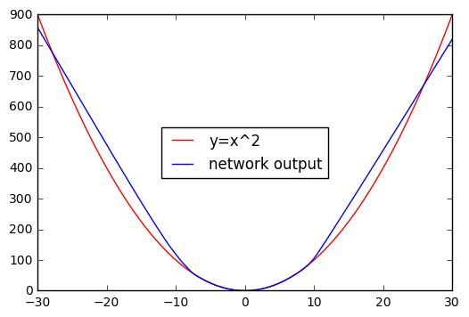
As you see, the network was tested on the interval [-30, +30], and it produced decent results. Now what happens if we increase the testing interval? Here you go:

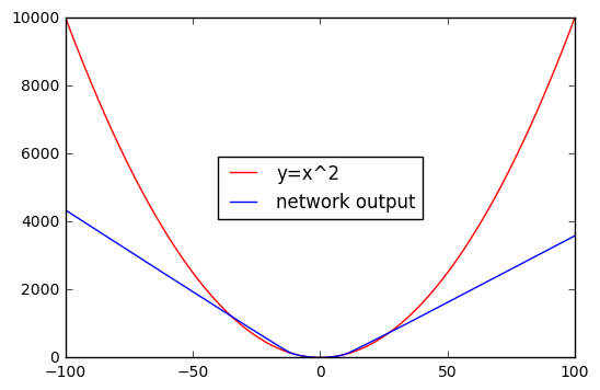
You can see now that the error increased drastically when we increased the testing interval. So why is that? Why is it that ANNs can do wonders but fails in finding the pattern of a basic square function? It’s because of extrapolation.

Interpolation vs Extrapolation Interpolation is an estimation of a value within two known values in a sequence of values (i.e [a,b] where a,b are finite numbers). Polynomial interpolation is a method of estimating values between known data points. When graphical data contains a gap, but data is available on either side of the gap or at a few specific points within the gap, interpolation allows us to estimate the values within the gap.

Extrapolation is an estimation of a value based on extending a known sequence of values or facts beyond the area that is certainly known. In a general sense, to extrapolate is to infer something that is not explicitly stated from existing information.

Approximating a polynomial function for an infinite range of values falls under Extrapolation, however, ANNs are suited for Interpolation. But why?

Let’s assume that we have a training set y with y∈ R. Can a neural network regression model extrapolate and return y_pred values outside the y range in a training set? Does it depend on the activation function or not?

The output neuron of the model is just ∑Θ[i]a[i], where Θ[i] — is the weight of i-th neuron on the previous hidden layer, and a[i] — is the value of the activation function of that neuron. If we use the logistic function then a ∈ [-1, +1]. Thus maximum possible y_pred=∑Θ[i], assuming that all “a”s reach their maximum value around 1. But if we use the linear activation function, which doesn’t have restrictions on the output values of a (a ∈ R) the model will return y_pred ∈ R, which can be outside the range of the training set. Does that mean the output is correct? No. Prediction will be less good in regions of the data that were not present in the training data. That’s why extrapolation is hard for Neural Networks.

So what now? Is that it? No, there are so many solutions to that problem. It won’t give you the accuracy of interpolating a neural network, but still, it’ll give you good results. One of the solutions is using a rectifier unit g(x)=max(0,x) as an activation function. It’s an unbounded but non-linear link function. It also keeps the nice “universal approximation” property of the neural network, but with unbounded outputs.

That was my first blog post. I really enjoyed writing this, and learned so much from it and I really hope you like it too. :)

Written on June 21st , 2018 by Mohammed Amarnah